
第四章 处理器架构
第四章 处理器架构
在第三章中学习的机器语言规则是在 x86-64 系列处理器环境之下的,如果是其他系列的处理器,第三章中的规则就不再适用了。
不同的处理器支持不同的指令和指令的字节级编码,它们统称为处理器的指令集体系结构 (Instruction-Set Architecture, ISA)
4.1 Y86-64 指令集体系结构
4.1.1 程序员可见的状态
Y86-64 程序中的每条指令都会读取或修改处理器状态的某些部分。这称为程序员可见状态,这里的”程序员”既可以是用汇编代码写程序的人,也可以是产生机器级代码的编译器。
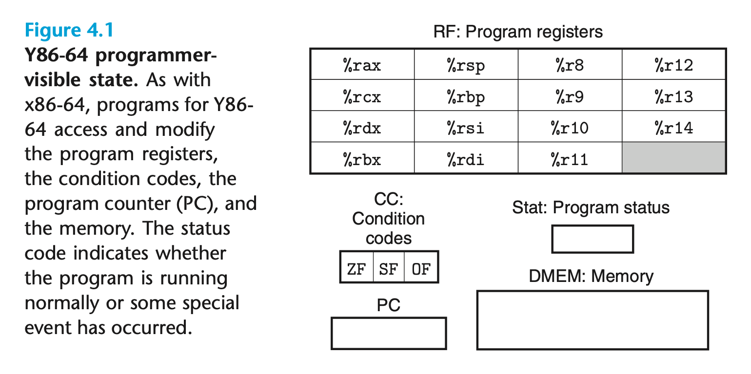
上图中的这些就是Y86-64中程序员可见状态:程序寄存器15个,条件位3个,状态位,program counter和内存
4.1.2 Y86-64 指令
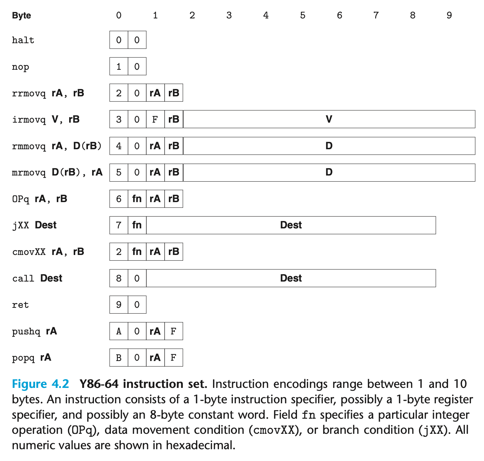
x86-64 的 movq 指令分成了 4 个不同的指令: irmovq、 rrmovq、 mrmovq 和 rmmovq, 分别显式地指明源和目的的格式。源可以是立即数(立、寄存器 (r)或内存 (m) 。指令 名字的第一个字母就表明了源的类型。目的可以是寄存器 (r)或内存 (m)。指令名字的第二个字母指明了目的的类型。
不允许从一个内存地址直接传送到另一个内存地址。另外,也不允许将立即数传送到内存。
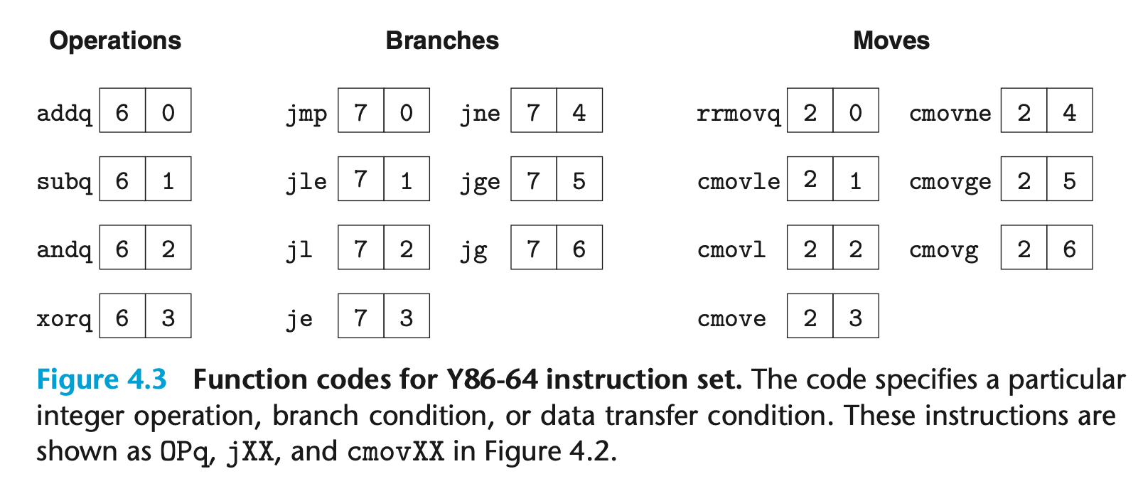
OPq包含 4 个整数操作指令,它们是 addq、 subq、 andq 和 xorq。 它 们只对寄存器数据进行操作,而 x86-64 还允许对内存数据进行这些操作。这些指令 会设置 3 个条件码 ZF、 SF 和 OF(零、符号和溢出)。
jXX包含7 个跳转指令,它们是 jmp、 jle、 jl、 je、 jne、 jge 和 jg。根据分支指令的类型和条件代码的设置来选择分支。
cmovXX包含 6 个条件传送指令: cmovle、 cmovl、 cmove、 cmovne、cmovge 和 cmovg
4.1.3 指令编码
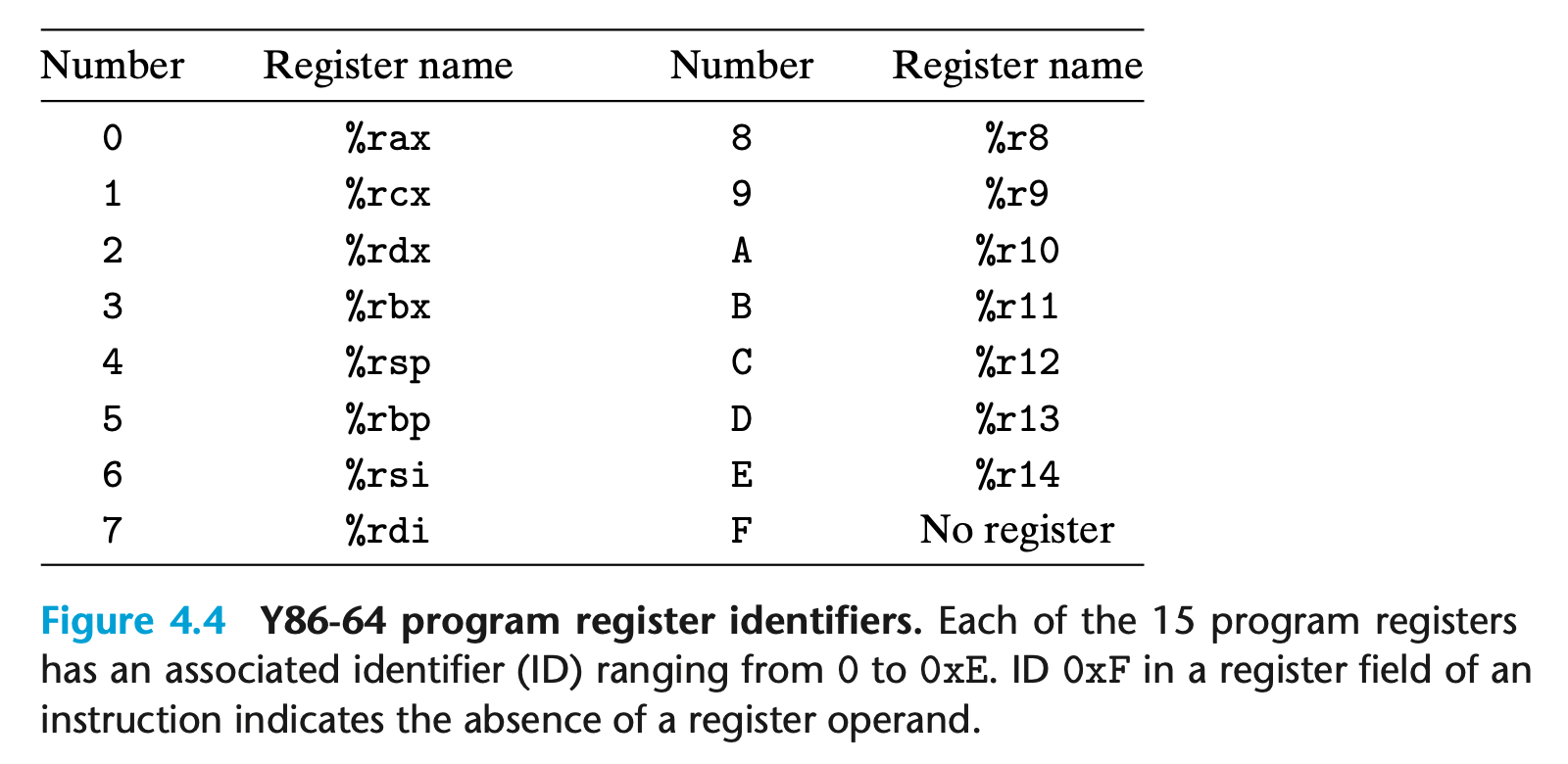
寄存器标识符 (register ID)
在Y86-64中,所有整数采用小端法编码。当指令按照反汇编格式书写时,这些字节就以相反的顺序出现。
例如,用十六进制来表示指令 rmrnovq %rsp, Ox123456789abcd(%rdx) 的字节编码。 从图 4-2 我们可以看到, rmmovq 的第 一 个字节为 40。源寄存器 %rsp 应该编码放在 rA 字段中,而基址寄存器 %rdx 应该编码放在 rB 字段中。根据图 4-4 中的寄存器编号,我 们得到寄存器指示符字节 42。最后,偏移量编码放在 8 字节的常数字中。首先在 0x123456789abcd 的前面填充上 0 变成 8 个字节,变成字节序列 00 01 23 45 67 89 ab cd。 写成按字节反序就是 cd ab 89 67 45 23 01 00。将它们都连接起来就得到指令的编码 4042cdab896745230100 。
Practice Problem 4.1
Determine the byte encoding of the Y86-64 instruction sequence that follows. The line .pos 0x100 indicates that the starting address of the object code should be 0x100.
1 | .pos 0x100 # Start code at address 0x100 |
1 | 0x100 30 f3 0f 00 00 00 00 00 00 00 |
4.1.4 Y86-64 Exceptions (异常)
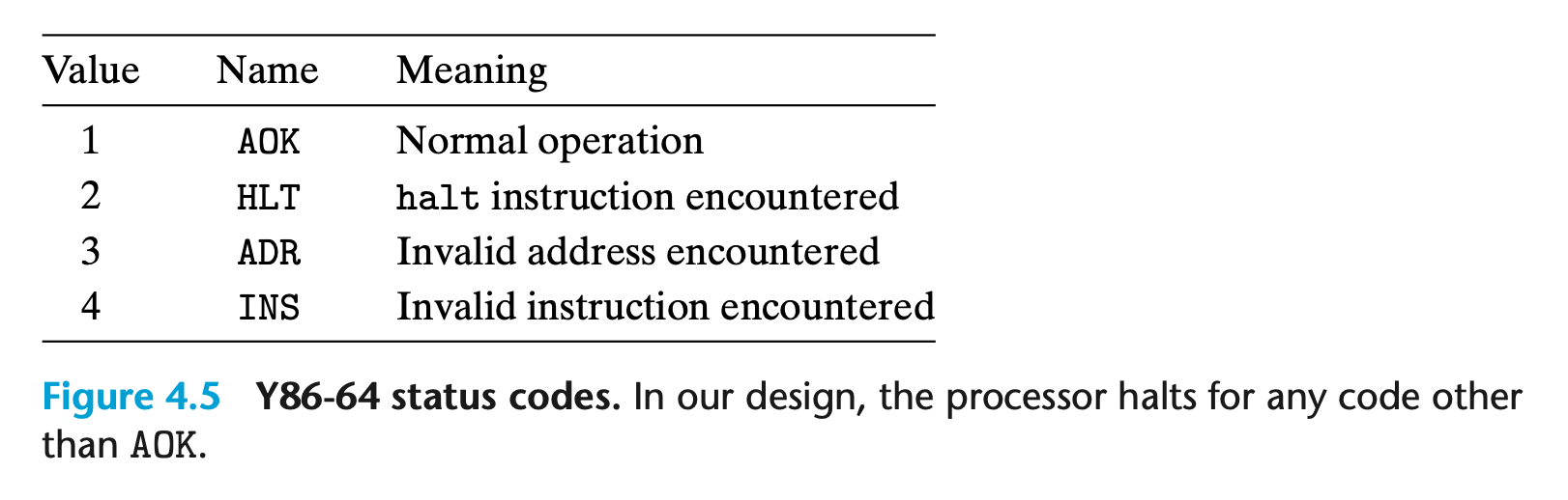
Y86-64 共有四个状态码,就是上图中的四个代码。第一个码表示一切正常,其他三个表明执行指令时出现了异常。
对于 Y86-64, 当遇到这些异常的时候,我们就简单地让处理器停止执行指令。在更完整的设计中,处理器通常会调用一个异常处理程序
(exception handler)
4.1.5 Y86-64 程序
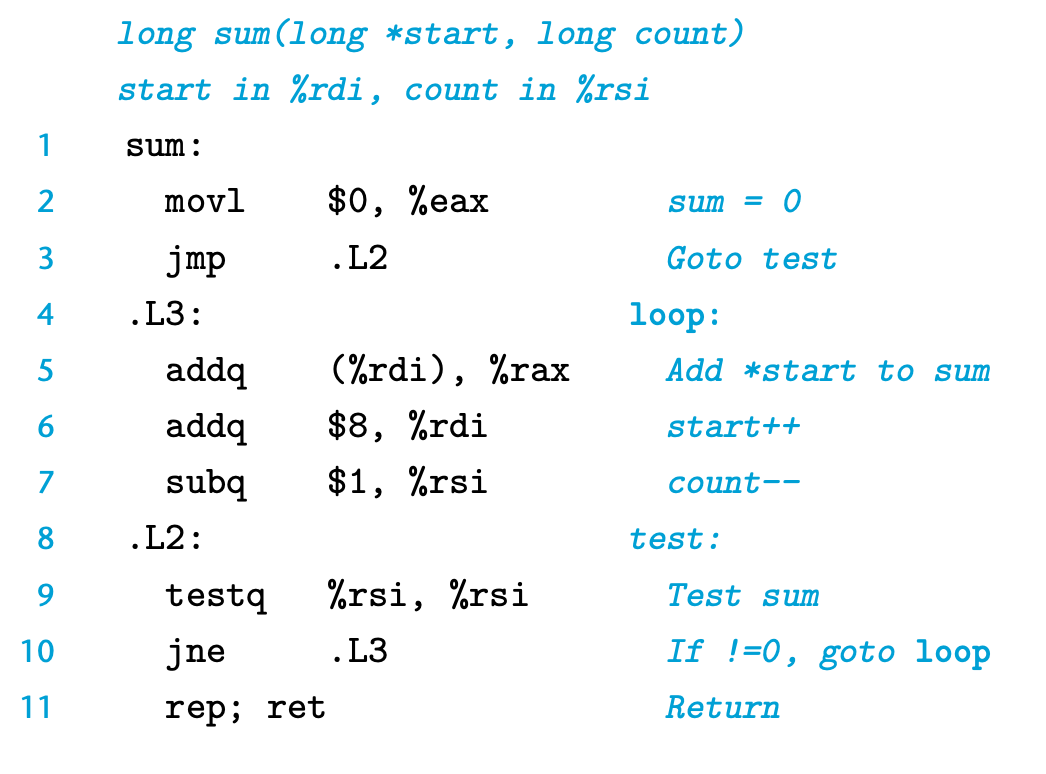
sum 函数C代码
1 | long sum(long *start, long count){ |
X86-64 代码
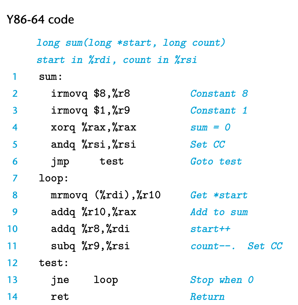
Y86-64 代码
下面的程序给出了用 Y86-64 汇编代码编写的一个完整的程序文件的例子。这个程序既包 括数据,也包括指令。伪指令 (directive)指明应该将代码或数据放在什么位置,以及如何对齐。这个程序详细说明了栈的放置、数据初始化、程序初始化和程序结束等问题。
1 | # Execution begins at address 0 |
Practice Problem 4.3
One common pattern in machine-level programs is to add a constant value to a register.With the Y86-64 instructions presented thus far, this requires first using an irmovq instruction to set a register to the constant, and then an addq instruction to add this value to the destination register. Suppose we want to add a new instruction iaddq with the following format:
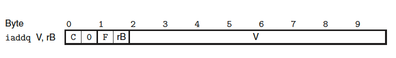
This instruction adds the constant value V to register rB.
Rewrite the Y86-64 sum function below to make use of the iaddq instruction. In the original version, we dedicated registers %r8 and %r9 to hold constant values. Now, we can avoid using those registers altogether.
1 | ;long sum(long *start, long count) |
改写版本
1 | ;long sum(long *start, long count) |
Practice Problem 4.4
Write Y86-64 code to implement a recursive product function rproduct, based on the following C code:
1 | long rproduct(long *start, long count){ |
1 | rproduct: |
Practice Problem 4.5
Modify the Y86-64 code for the sum function to implement a function absSum that computes the sum of absolute values of an array. Use a conditional jump instruction within your inner loop.
1 | # long sum(long *start, long count) |
1 | # long sum(long *start, long count) |
Practice Problem 4.6
Modify the Y86-64 code for the sum function to implement a function absSum that computes the sum of absolute values of an array. Use a conditional move instruction within your inner loop.
1 | # long sum(long *start, long count) |
4.1.6 一些 Y86-64 指令的详情
两个特别的 Y86-64 指令的组合需要特别注意一下。
pushq 指令会把栈指针减 8, 并且将一个寄存器值写入内存中。因此,当执行 pushq %rsp 指令时,处理器的行为是不确定的,因为要入栈的寄存器会被同一条指令修改。通常有两种不同的约定: 1)压入 %rsp 的原始值, 2)压入减去 8 的 %rsp 的值。
Practice Problem 4.7
Let us determine the behavior of the instruction pushq %rsp for an x86-64 processor.We could try reading the Intel documentation on this instruction, but a simpler approach is to conduct an experiment on an actual machine. The C compiler would not normally generate this instruction, so we must use hand-generated assembly code for this task. Here is a test function we have written (Web Aside asm:easm on page 214 describes how to write programs that combine C code with handwritten assembly code):
1 | .text |
In our experiments, we find that function pushtest always returns 0. What does this imply about the behavior of the instruction pushq %rsp under x86-64?
压入 %rsp 的原始值
对 popq %rsp 指令也有类似的歧义。可以将 %rsp 置为从内存中读出的值,也可以置为加了增量后的栈指针
Practice Problem 4.8
The following assembly-code function lets us determine the behavior of the instruction popq %rsp for x86-64:
1 | .text |
We find this function always returns 0xabcd. What does this imply about the behavior of popq %rsp? What other Y86-64 instruction would have the exact same behavior?
将 %rsp 置为从内存中读出的值
4.2 逻辑设计和硬件控制语言 HCL
HCL (Hardware Control Language, 硬件控制语言)
大多数现代电路技术都是用信号线上的高电压或低电压来表示不同的位值 。 在当前的技术中,逻辑 1 是用 1.0 伏特左右 的高电压表示的,而逻辑 0 是用 0.0 伏特左右的低电压表示的。
要实现一个数字系统需要三个主要的组成部分:
- combinational logic to compute functions on the bits
- memory elements to store bits
- clock signals to regulate the updating of the memory elements
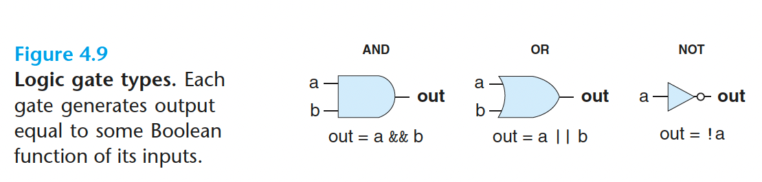
4.2.1 逻辑门
HCL中的逻辑运算
| 逻辑运算 | 符号 | ||
|---|---|---|---|
| and | && | ||
| or | \ | \ | |
| not | ! |
4.2.2 组合电路和 HCL 布尔表达式
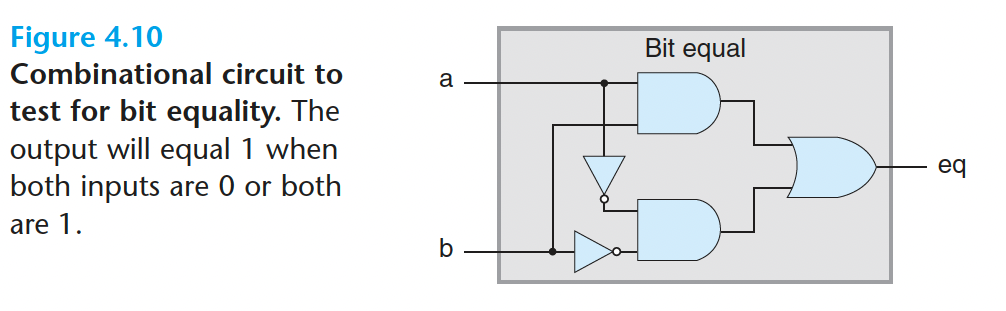
1 | bool eq = (a&&b)||(!a&&!b); |
Practice Problem 4.9
Write an HCL expression for a signal xor, equal to the exclusive-or of inputs a and b. What is the relation between the signals xor and eq defined above?
1 | bool xor = !((a&&b)||(!a&&!b)); |
multiplexor 多路复用器 MUX:
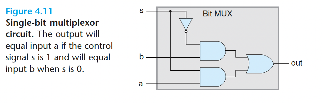
1 | bool out = (s && a) || (!s && b); |
4.2.3 字级的组合电路和HCL整数表达式
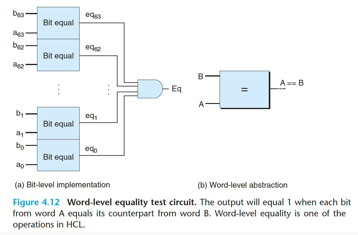
上图所示的电路的函数可以在字级上表达成:
1 | bool Eq = (A == B); |
在 HCL 中,我们将所有字级的信号都声明为 int, 不指定字的大小。
字级的多路复用器:
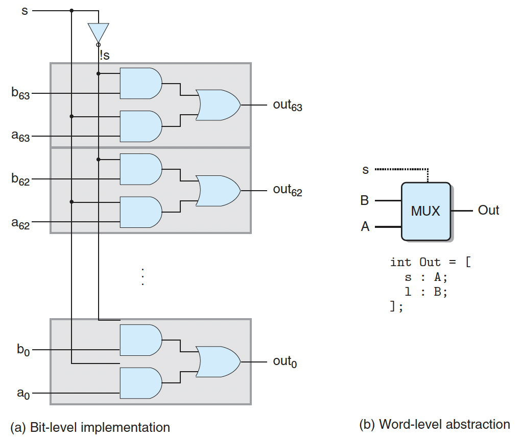
在HCL中,字级的多路复用器用情况表达式(case expression)描述。它的通用格式如下:
1 | [ |
这个表达式包含一系列的情况,每种情况 i 都有一个布尔表达式 $select_i$ , 和一个整数表达式 $expr_i$, 前者表明什么时候该选择这种情况,后者指明的是得到的值。
同 C 的 switch 语句不同,我们不要求不同的选择表达式之间互斥。从逻辑上讲,这些选择表达式是顺序求值的,且第一个求值为1 的情况会被选中。
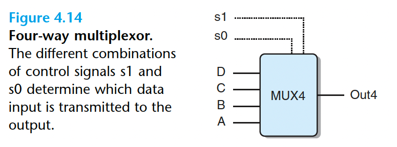
四路复用器的HCL代码:
1 | [ |
假设我们想设计一个逻辑电路来找一组字 A、B 和 C 中的最小值,
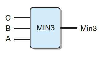
1 | word Min3 = [ |
Practice Problem 4.11
The HCL code given for computing the minimum of three words contains four comparison expressions of the form $X <= Y$ . Rewrite the code to compute the same result, but using only three comparisons.
1 | word Min3 = [ |
Practice Problem 4.12
Write HCL code describing a circuit that for word inputs A, B, and C selects the median of the three values. That is, the output equals the word lying between the minimum and maximum of the three inputs.
1 | word Median3 = [ |
算术/逻辑单元(ALU):
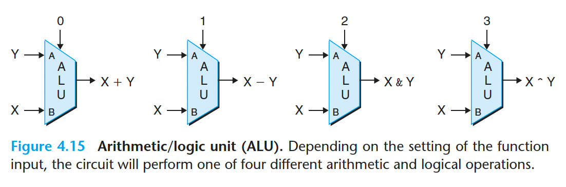
根据输入来决定执行的操作(加减乘除)
4.2.4 集合关系
判断集合关系的通用格式是:
1 | iexpr in {iexpr1,iexpr2,...,iexprk} |
比如
1 | bool s1 = code in { 2, 3 }; |
4.2.5 存储器和时钟
考虑两类存储器设备:
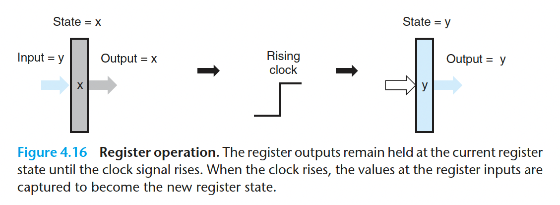
- 时钟寄存器(简称寄存器)存储单个位或字。时钟信号控制寄存器加载输入值。
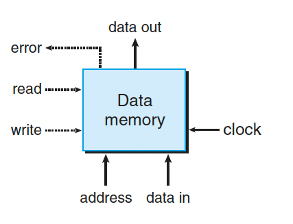
- 随机访问存储器(简称内存)存储多个字,用地址来选择该读或该写哪个字。
大多数时候,寄存器都保待在稳定状态(用 x 表示),产生的输出等于它的当前状态。在时钟的上升沿,寄存器的内容会更新,输出也会更新(为 y)。
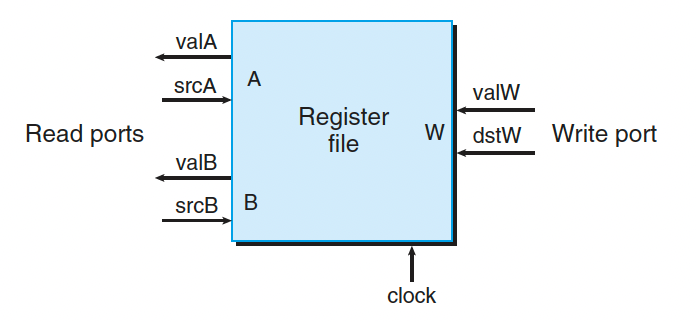
寄存器文件 register file:
随机访问存储器:
4.3 Sequential (SEQ) Y86-64 Implementations
4.3.1 Organizing Processing into Stages
通常,处理一条指令包括很多操作。将它们组织成某个特殊的阶段序列,即使指令的动作差异很大,但所有的指令都遵循统一的序列。
下面是关于各个阶段以及各阶段内执行操作的简略描述:
fetch
取指阶段从内存读取指令字节,地址为程序计数器 (PC) 的值。
decode
译码阶段从寄存器文件读入最多两个操作数,得到值 valA 和/或 valB
execute
在执行阶段,算术/逻辑单元 (ALU) 要么执行指令指明的操作(根据 ifun的值),计算内存引用的有效地址,要么增加或减少栈指针。
memory
访存阶段可以将数据写入内存,或者从内存读出数据。
write back
写回阶段最多可以写两个结果到寄存器文件。
PC update
将 PC 设置成下一条指令的地址。
Practice Problem 4.13
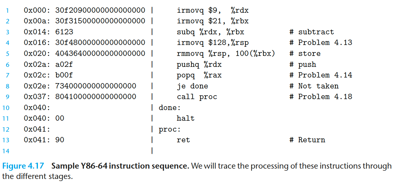
Fill in the right-hand column of the following table to describe the processing of the irmovq instruction on line 4 of the object code in Figure 4.17:
| stage | genericirmovq V,rB |
specificirmovq $128,%rsp |
|---|---|---|
| Fetch | icode:ifun $\leftarrow$ $M_1[PC]$ rA:rB $\leftarrow$ $M_1[PC+1]$ valC $\leftarrow$ $M_8[PC+2]$ valP $\leftarrow$ $PC+10$ |
icode:ifun $\leftarrow$ $M_1[0x16]=3:0$ rA:rB $\leftarrow$ $M_1[0x17]=f:4$ valC $\leftarrow$ $M_8[0x18]=0x80$ valP $\leftarrow$ $PC+10=0x20$ |
| Decode | ||
| Execute | valE = 0+valC | valE = 0+valC=0x80 |
| Memory | ||
| Write back | R[rB] $\leftarrow$ valE | R[%rsp] $\leftarrow$ valE=0x80 |
| PC update | PC $\leftarrow$ valP | PC $\leftarrow$ valP=0x20 |
rmmovq 和 mrmvoq 操作顺序
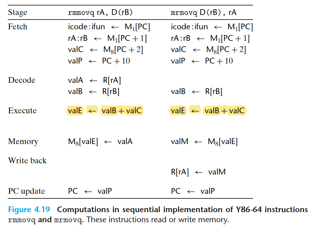
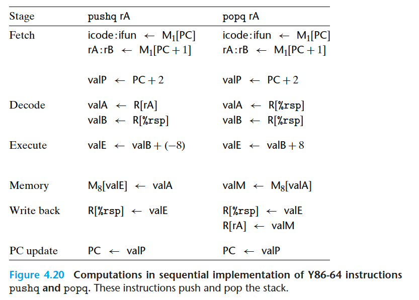
pushq 和 popq 的操作顺序
Practice Problem 4.14
Fill in the right-hand column of the following table to describe the processing of the popq instruction on line 7 of the object code in Figure 4.17.
| stage | genericpopq rA |
specificpopq %rax |
|---|---|---|
| Fetch | icode:ifun $\leftarrow$ $M_1[PC]$ rA:rB $\leftarrow$ $M_1[PC+1]$ valP $\leftarrow$ $PC+2$ |
icode:ifun $\leftarrow$ $M_1[0x2c]=b:0$ rA:rB $\leftarrow$ $M_1[0x2d]=0:f$ valP $\leftarrow$ $PC+2=0x2e$ |
| Decode | valA $\leftarrow$ R[%rsp] valB $\leftarrow$ R[%rsp] |
valA $\leftarrow$ R[%rsp]=120 valB $\leftarrow$ R[%rsp]=120 |
| Execute | valE = valB+8 | valE = valB+8=128 |
| Memory | valM $\leftarrow$ $M_8[valA]$ | valM $\leftarrow$ $M_8[valA]=9$ |
| Write back | R[rA] $\leftarrow$ valM R[%rsp] $\leftarrow$ valE |
R[rA] $\leftarrow$ valM=9 R[%rsp] $\leftarrow$ valE=128 |
| PC update | PC $\leftarrow$ valP | PC $\leftarrow$ valP=0x2e |
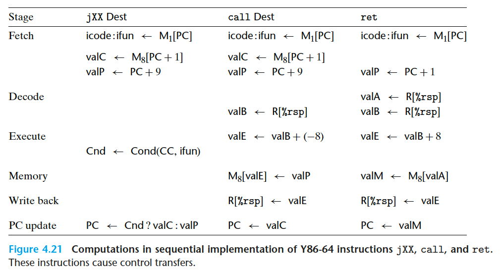
各类控制转移指令的操作顺序:
Practice Problem 4.17
We can see by the instruction encodings (Figures 4.2 and 4.3) that the rrmovq instruction is the unconditional version of a more general class of instructions that include the conditional moves. Show how you would modify the steps for the rrmovq instruction below to also handle the six conditional move instructions. You may find it useful to see how the implementation of the jXX instructions (Figure 4.21) handles conditional behavior.
| stage | genericcmovXX rA,rB |
|---|---|
| Fetch | icode:ifun $\leftarrow$ $M_1[PC]$ rA:rB $\leftarrow$ $M_1[PC+1]$ valP $\leftarrow$ $PC+2$ |
| Decode | valA $\leftarrow$ R[rA] |
| Execute | Cnd $\leftarrow$ Cond(CC,ifun) valE $\leftarrow$ Cnd ? valA : valE |
| Memory | |
| Write back | R[rB] $\leftarrow$ valE |
| PC update | PC $\leftarrow$ valP |
我们创建了一个统一的框架,能处理所有不同类型的 Y86-64 指令 。
现在的任务是创建硬件设计来实现这些阶段,并把它们连接起来。
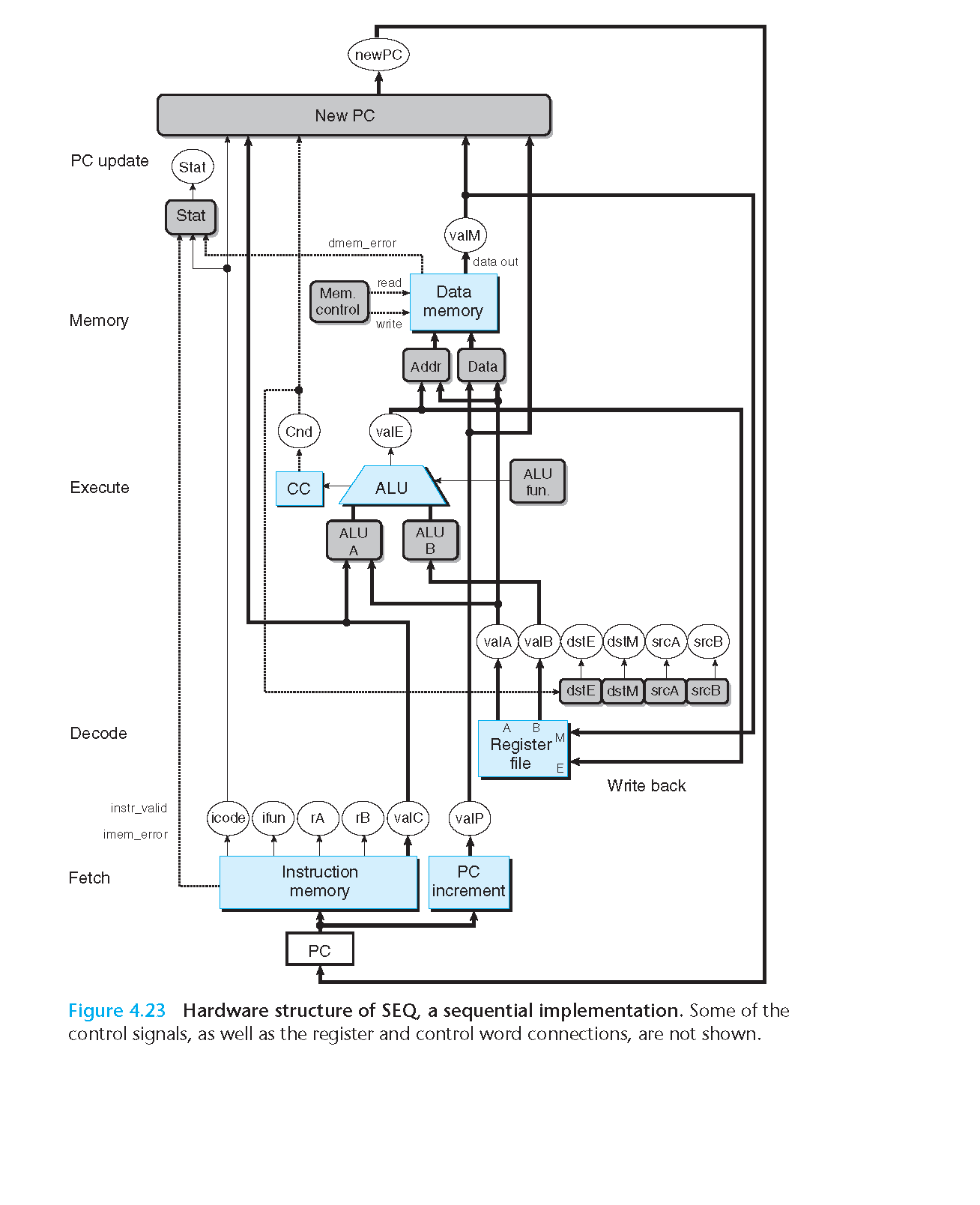
4.3.2 SEQ 硬件结构
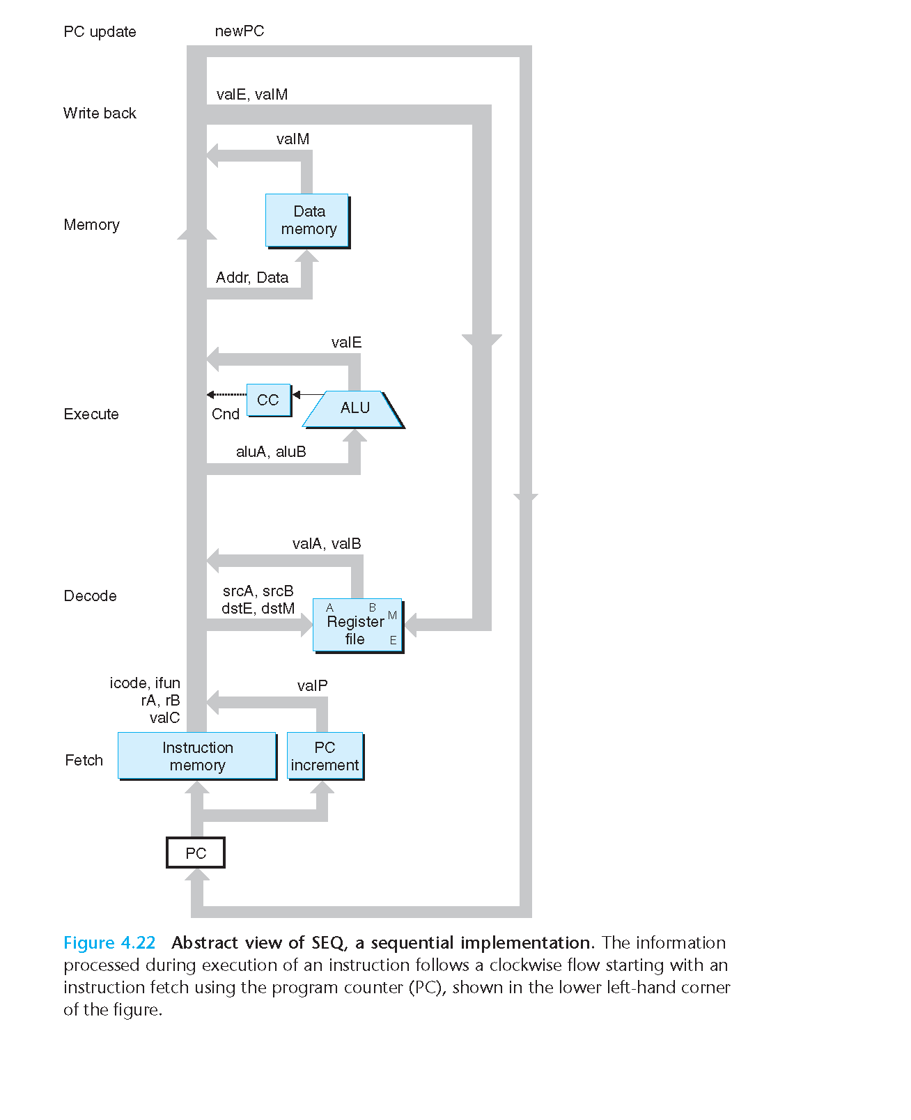
上面是SEQ硬件系统的抽象图
下面的是更加详细的图
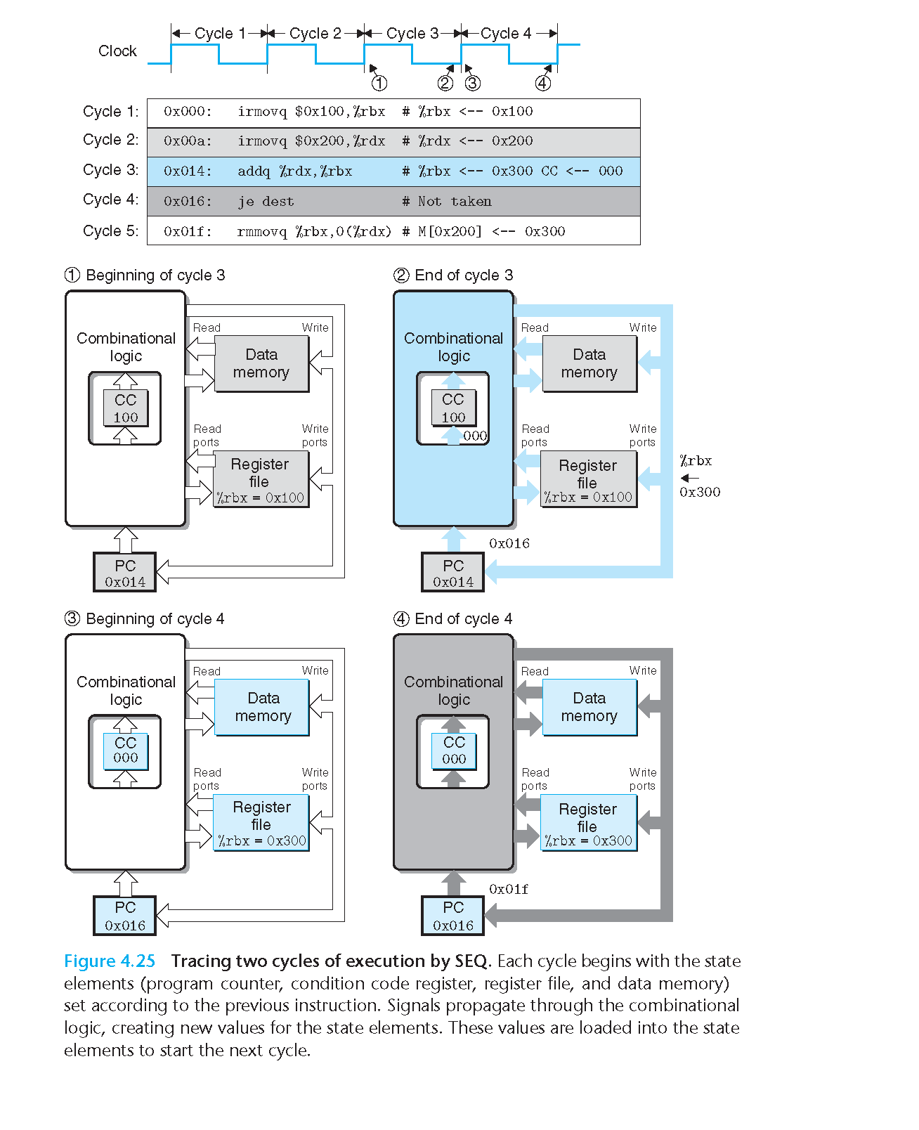
4.3.3 SEQ 的时序
4.3.4 SEQ Stage Implementations
fetch阶段
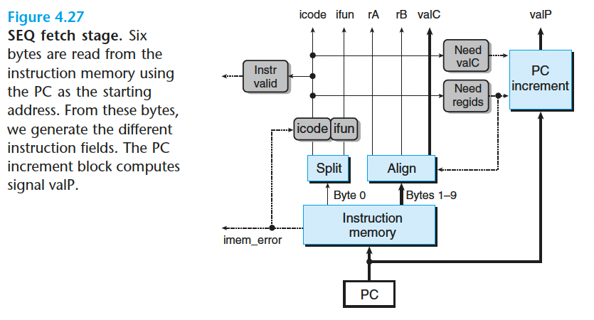
instr_valid
这个字节对应于一 个合法的 Y86-64 指令吗?这个信号用来 发现不合法的指令。
need_regids
这个指令包括一个寄存器指示符字节吗?
need_valC
这个指令包括一个常数字吗?
need_regids 的 HCL 描述只是确定了 icode 的值是否为一条带有寄存器指示值字节的指令。
1 | bool need_regids = icode in { IRRMOVQ,IOPQ,IPUSHQ,IPOPQ, |
Practice Problem 4.19
Write HCL code for the signal need_valC in the SEQ implementation.
1 | bool need_valC = in { IIRMOVQ,IRMMOVQ,IMRMOVQ,IJXX,ICALL }; |
- decode 和 write back 阶段
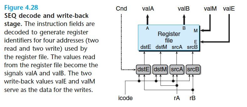
寄存器 ID srcA 表明应该读哪个寄存器以产生 valA。所需要的值依赖于指令类型,如图 4-18~ 图 4-21 中译码阶段第一行中所示 。 将所有这些条目都整合到一个计算中就得到下面的 srcA 的 HCL 描述 (回想 RRSP 是 %rsp 的寄存器 ID):
1 | word srcA = [ |
Practice Problem 4.20
The register signal srcB indicates which register should be read to generate the signal valB. The desired value is shown as the second step in the decode stage in Figures 4.18 to 4.21. Write HCL code for srcB.
1 | word srcB = [ |
寄存器 ID dstE 表明写端口 E 的目的寄存器,计算出来的值 valE 将放在那里。
如果我们暂时忽略条件移动指令,综合所有不同指令的目的寄存器,就得到下面的 dstE 的 HCL 描述:
1 | WARNING: Conditional move not implemented correctly here |
Practice Problem 4.21
Register ID dstM indicates the destination register for write port M, where valM, the value read from memory, is stored. This is shown in Figures 4.18 to 4.21 as the second step in the write-back stage. Write HCL code for dstM.
1 | word dstM = [ |
Practice Problem 4.22
只有 popq 指令会同时用到寄存器文件的两个写端口。对于指令 popq %rsp, E 和 M 两个写端口会用到同一个地址,但是写入的数据不同。为了解决这个 冲突,必须对两个写端口设立一个优先级,这样一来,当同一个周期内两个写端口都 试图对一个寄存器进行写时,只有较高优先级端口上的写才会发生。那么要实现练习 题 4. 8 中确定的行为,哪个端口该具有较高的优先级呢?
M端口
因为这条命令把 M[%rsp] 的内容写进 %rsp
- execute 阶段
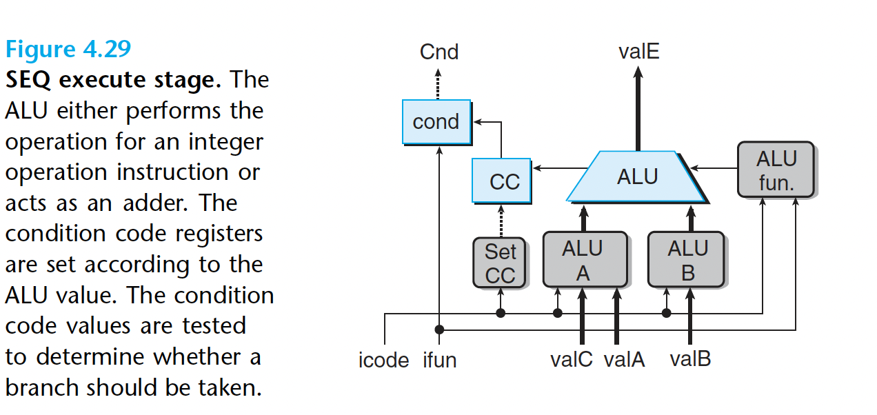
执行阶段的第一步就是每条指令的 ALU 计算。列出的操作数 aluB 在前面,后面是 aluA
因此我们可以用下面的方式来表达产生 aluA 的控 制块的行为:
1 | word aluA = [ |
Practice Problem 4.23
Based on the first operand of the first step of the execute stage in Figures 4.18 to 4.21, write an HCL description for the signal aluB in SEQ.
valB: opq, rmmovq, mrmovq, pushq, popq, call, ret
0: rrmovq, irmovq,
1 | word aluB = [ |
- memory阶段
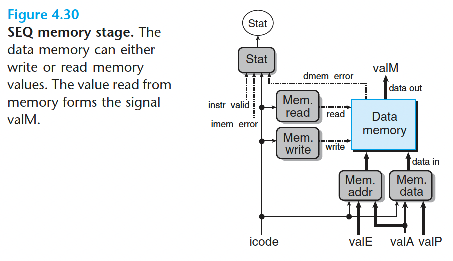
可以 看到内存读和写 的 地址 总是 valE 或 valA。这个块 用 HCL 描述 就是:
1 | word mem_addr = [ |
- update PC 阶段
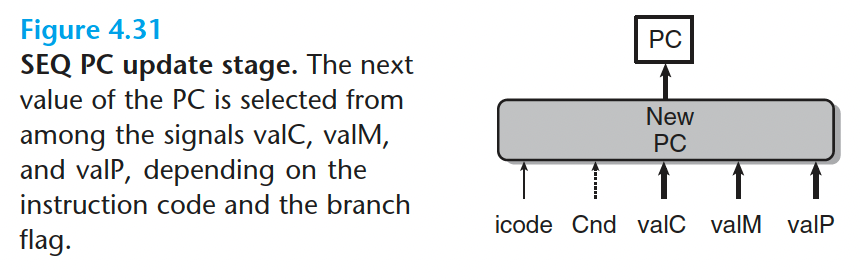
1 | word new_pc = [ |
4.4 流水线 (pipeline) 的通用原理
流水线化的一个重要特性就是提高了系统的吞吐量 (throughput), 不过它也会轻微地增加延迟 (latency),
4.4.1 计算流水线
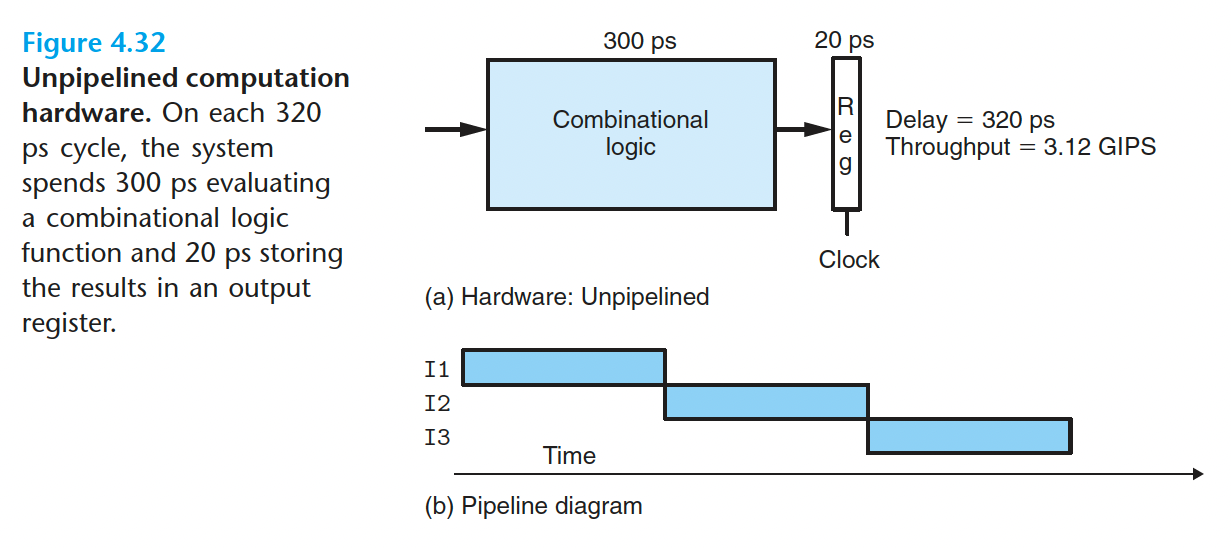
上面这幅图是未流水线化的硬件,执行每个指令需要$300+20=320ps$,每皮秒执行$1/320=3.125*10^{-3}$条指令,所以
再看看流水化的硬件
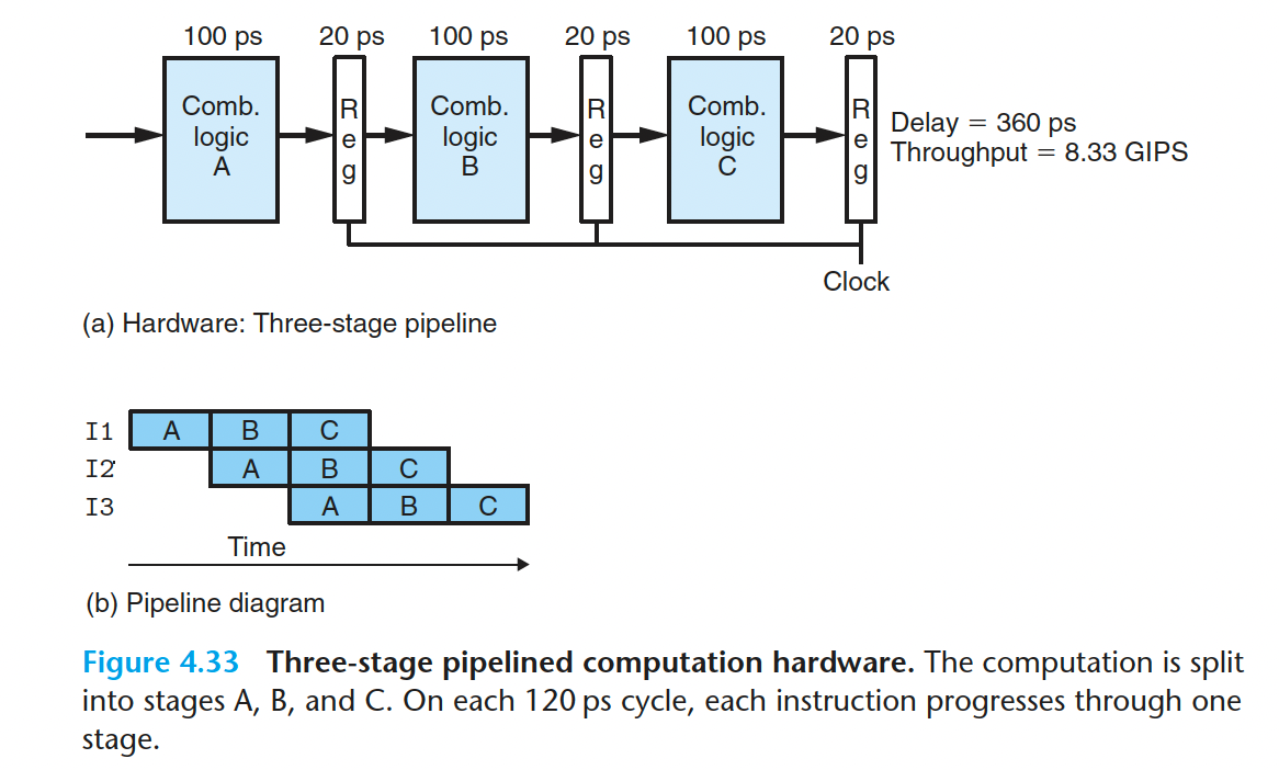
通过把一个指令分成固定的几个阶段,每个时钟中期内可以执行多个不同的阶段,虽然单条指令的执行时间变长了(360ps),但是处理器的吞吐量变大了(8.33 GIPS)
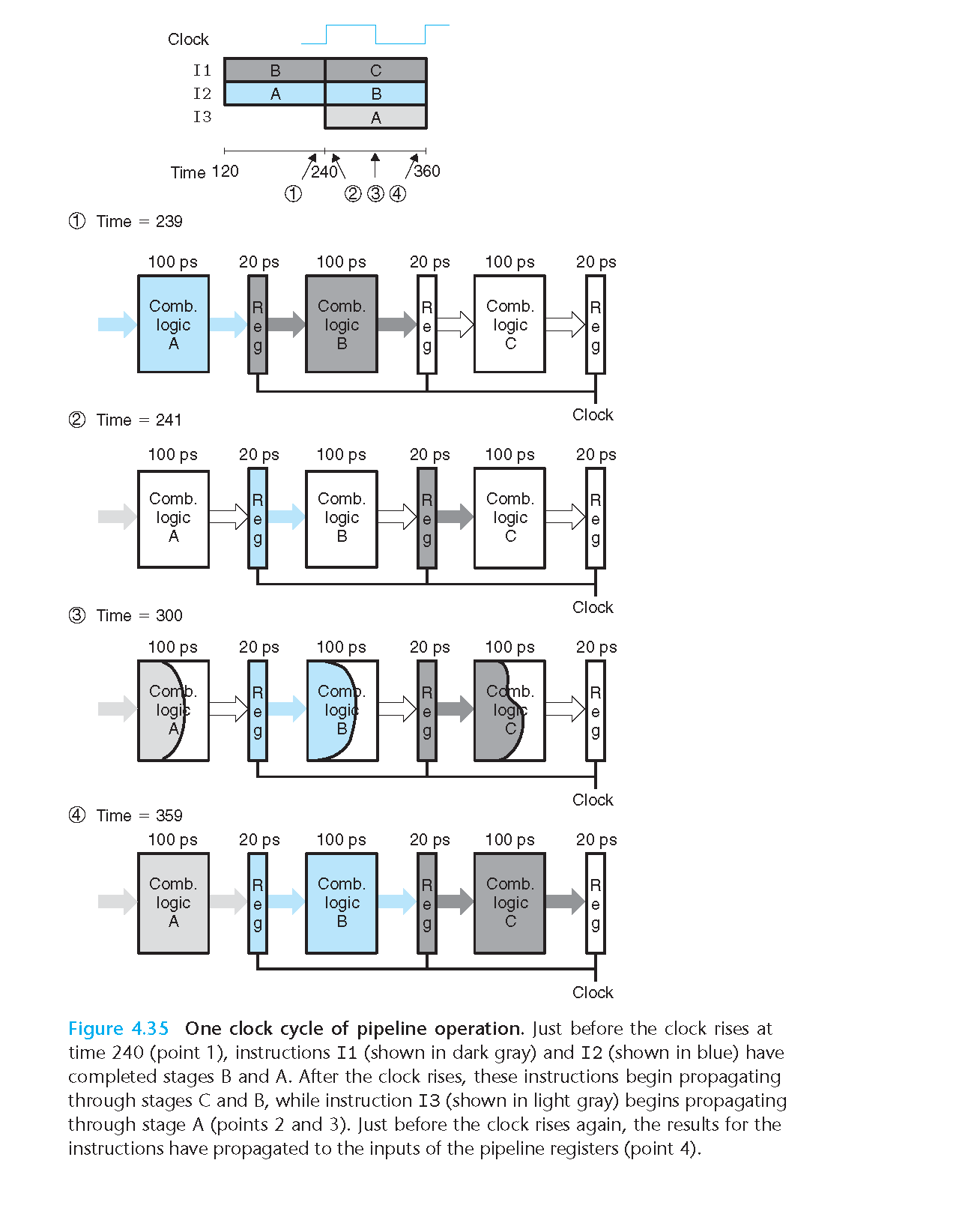
4.4.2 流水线操作的详细说明
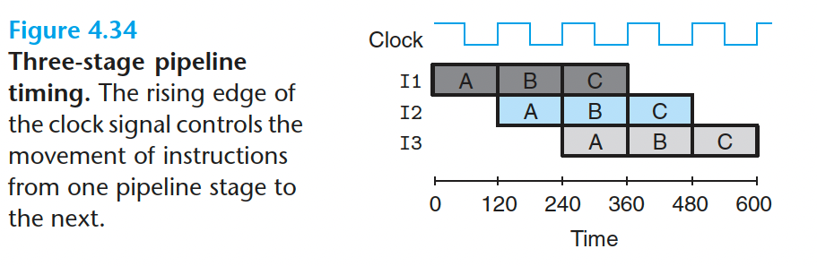
对240~360ps间流水操作的追踪:
4.4.3 流水线的局限性
下面这些因素会导致流水线效率降低
- 不一致的划分
一条指令划分成不同的阶段,各个阶段执行的时间并不都是相等的。这样的流水线会导致某些阶段赋闲,就像这样
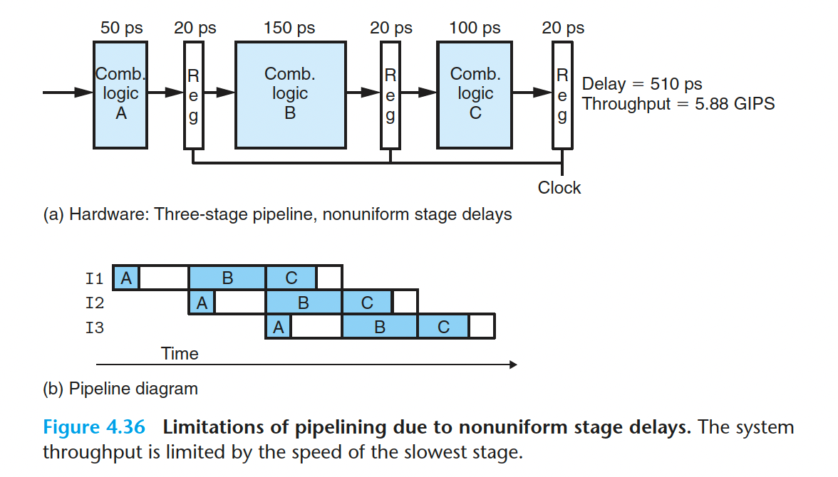
在这个图里,I2 的A阶段总会空闲100ps,同样的,I2 的C阶段总会空闲50ps,这是白白浪费时间
Practice Problem 4.28
Suppose we analyze a combinational logic and determine that it can be separated into a sequence of six blocks, named A to F, having delays of 80, 30, 60, 50, 70, and 10 ps, respectively, illustrated as follows:
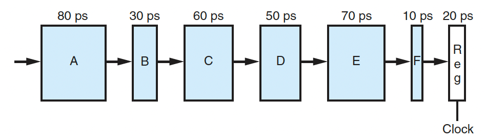
We can create pipelined versions of this design by inserting pipeline registers between pairs of these blocks. Different combinations of pipeline depth (how many stages) and maximum throughput arise, depending on where we insert the pipeline registers. Assume that a pipeline register has a delay of 20 ps.
A. Inserting a single register gives a two-stage pipeline. Where should the register be inserted to maximize throughput?What would be the throughput and latency?
5.26 GIPS, 380ps latency
B. Where should two registers be inserted to maximize the throughput of a three-stage pipeline? What would be the throughput and latency?
7.69 GIPS, 390ps latency
C. Where should three registers be inserted to maximize the throughput of a 4-stage pipeline?What would be the throughput and latency?
9.09 GIPS, 440ps latency
D. What is the minimum number of stages that would yield a design with the maximum achievable throughput? Describe this design, its throughput, and its latency.
10 GIPS, 500ps latency
- 流水线过深,受益反而下降
4.4.4 带反馈的流水线系统
到目前为止,我们只考虑一种系统,其中传过流水线的对象,相互都是完全独立的。但是,对于像 x86-64 或 Y86-64 这样执行机器程序的系统来 说,相邻指令之间很可能是相关的。
可能是下面这样的数据相关(data dependency)
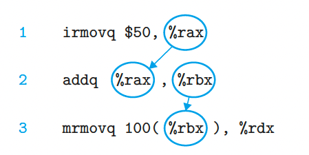
也有可能是控制相关(control dependency)
在我们的 SEQ 设 计中,这些相关都是由反馈路径来解决的。这些反馈将更新了的 寄存器值向下传送到寄存器文件,将新的 PC 值向下传送到 PC 寄存器。
在带有相关性的指令系统中引入流水线可能会带来问题:
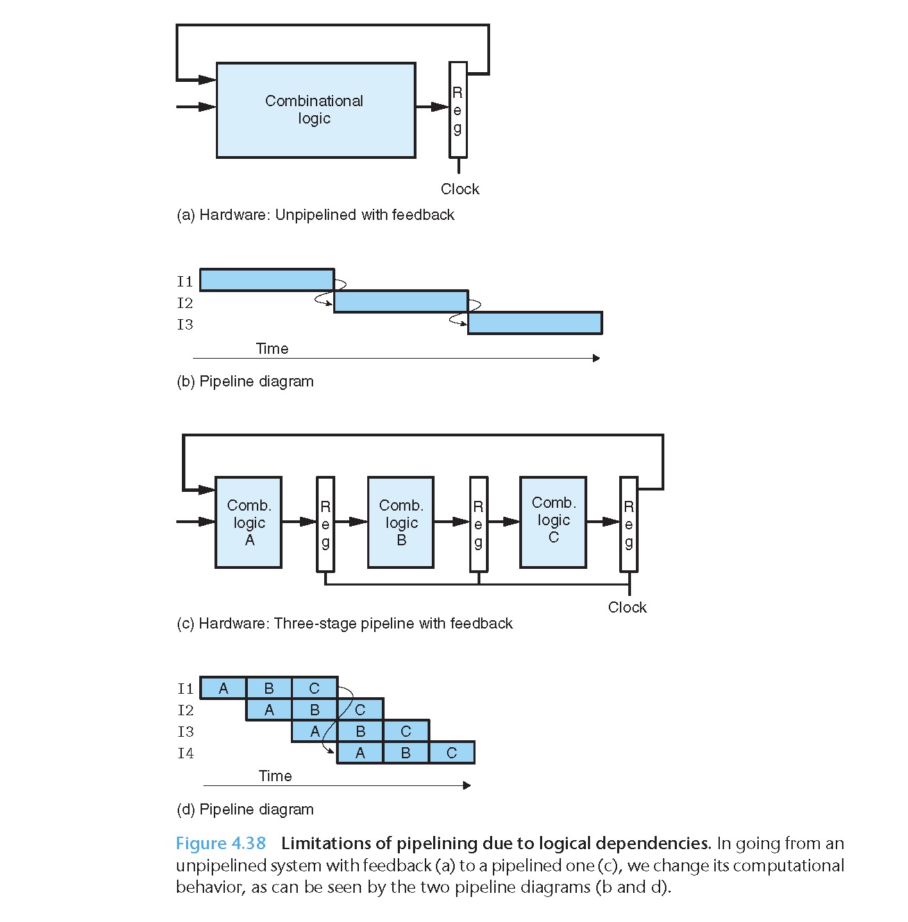
可以很明显的看到,原本(未流水化)传给紧邻着下一条的反馈信号在流水化后传递给了 I4
所以在设计 Y86-64 处理器的流水线时必须正确处理反馈的影响。
4.5 Y86-64 的流水线实现
4.5.1 SEQ+: 重新安排计算阶段
我们移动 PC 阶段,使得它的逻辑在时钟周期开始时活动,使它计算当前指令的 PC 值。改进后的设计称为 SEQ+
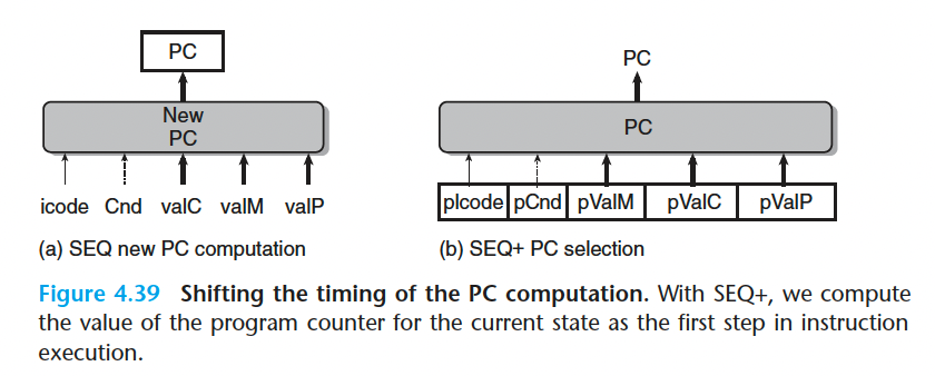
SEQ 到 SEQ+ 中对状态单元的改变是一种很通用的改进的例子,这种改进称为电路 重定时(circuit retiming)。重定时改变了一个系统的状态表示,但是并不改变它的逻辑行为 。 通常用它来平衡 一 个流水线系统中各个阶段之间的延迟。
4.5.2 插入流水线寄存器
我们要在 SEQ+ 的各个阶段之间插入流水线寄存器,并对信号重新排列,得到 PIPE- 处理器,这里的 “-” 代表这个处理器和最终的处理器设计相比,性能要差一点。
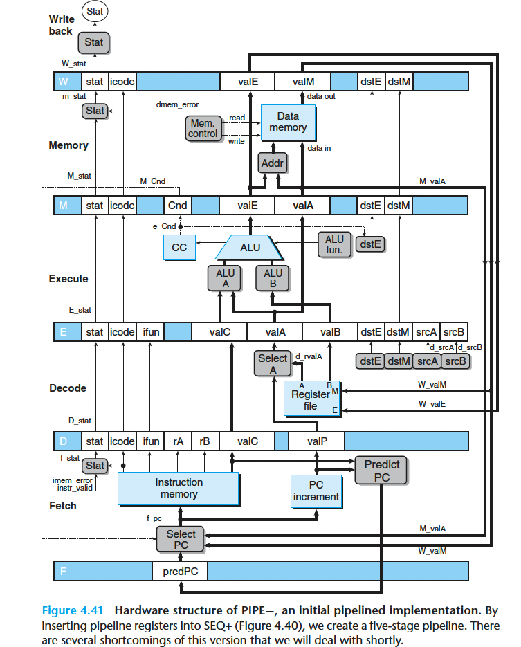
流水线寄存器的标号:
F 保存程序计数器的预测值
D 位于取指和译码阶段之间 。 它保存关于最新取出的指令的信息,即将由译码阶段进行处理。
E 位于译码和执行阶段之间 。 它保存关千最新译码的指令和从寄存器文件读出的值的信息,即将由执行阶段进行处理。
M 位于执行和访存阶段之间 。 它保存最新执行的指令的结果,即将由访存阶段进行处理 。 它还保存关于用于处理条件转移的分支条件和分支目标的信息。
W 位于访存阶段和反馈路径之间,反馈路径将计算出来的值提供给寄存器文件写,而当完成 ret 指令时 ,它还要向 PC 选择逻辑提供返回地址 。
4.5.3 对信号进行重新排列和标号
4.5.4 预测下一个 PC
在本书的设计中,总是预测选择了分支
4.5.5 流水线冒险
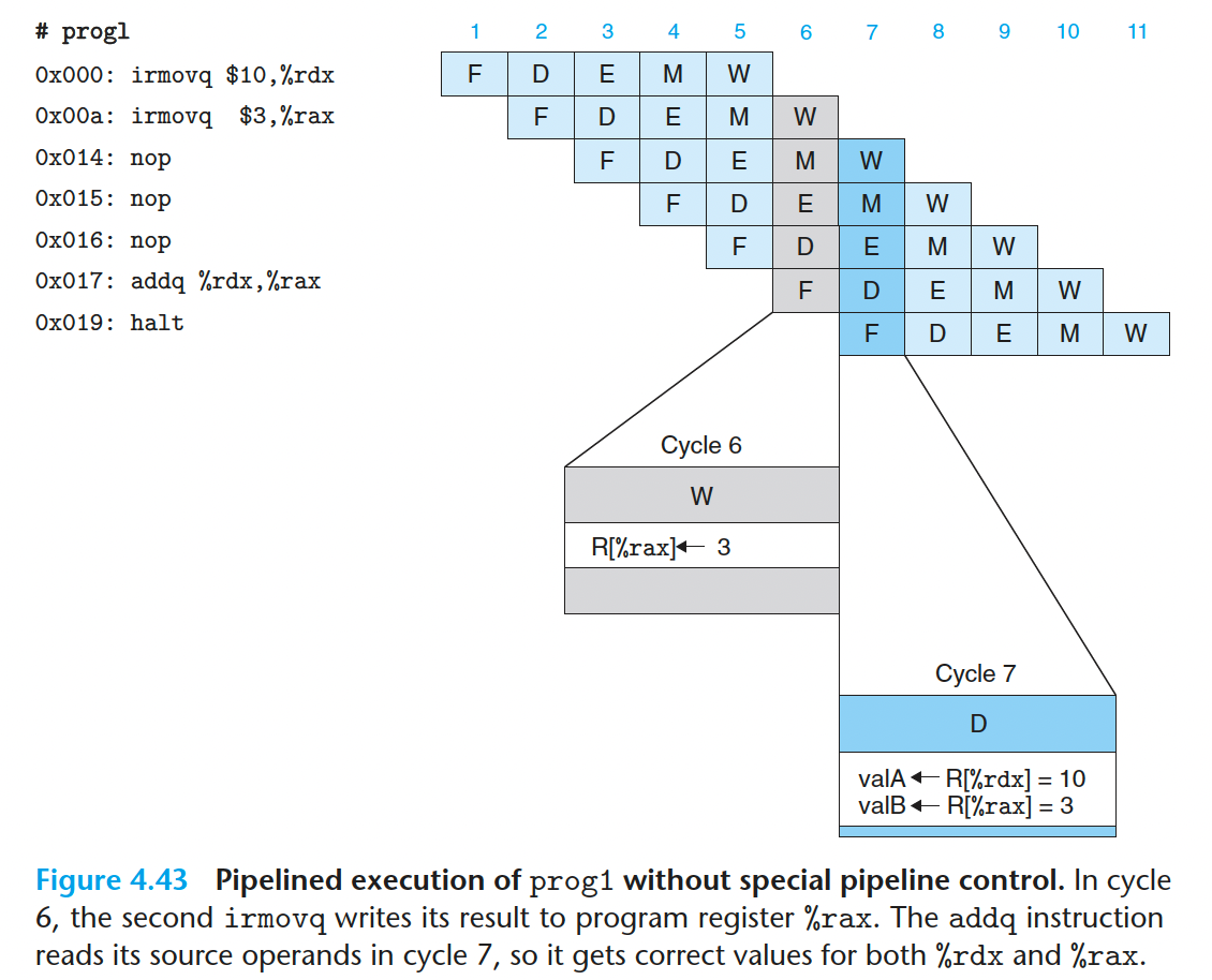
图 4-43 描述的是 PIPE- 处理器处理 progl 指令序列的情况。
在这个例子中,由于在周期7开始的时候,两个 irmovq 指令都完成了写回阶段,所以 周期7 的 D 解码阶段可以读到正确的值
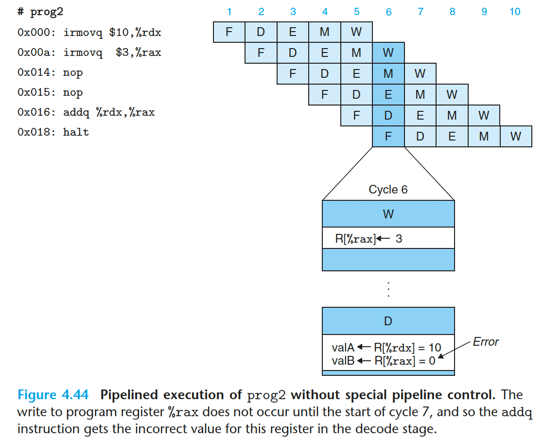
但是,如果去掉三条 nop 指令,执行 addq 之前就没有足够的时间完成两个 irmovq 指令的写回阶段了,那 addq的解码阶段就会得到错误的结果,就像下面这样:
- 用暂停来避免数据冒险
暂停 (stalling)是避免冒险的一种常用技术,暂停时,处理器会停止流水线中一条或多 条指令,直到冒险条件不再满足。
- 用转发来避免数据冒险
PIPE- 的设计是在译码阶段从寄存器文件中读入源操作数,但是对这些源寄存器的写有可能要在写回阶段才能进行。与其暂停直到写完成,不如简单地将要写的值传到流水线寄存器 E 作为源操作数。
这种将结果值直接从一个流水线阶段传到较早阶段的技术称为数据转发 (data forwarding, 或简称转发,有时称为旁路 (bypassing))。
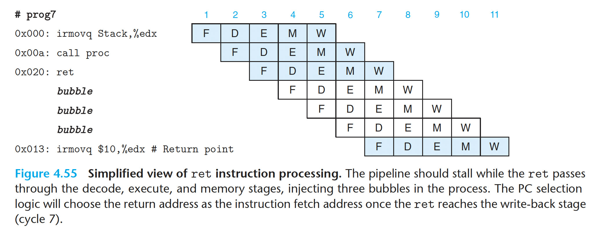
我们应该在ret执行到译码阶段开始插入气泡,接连插入三个,这样位于 0x013 位置处的 irmovq 指令才能执行。因为只有 ret 执行完写回阶段,PC 才能被设置为 0x013 ,也就是 irmovq 所在的地址
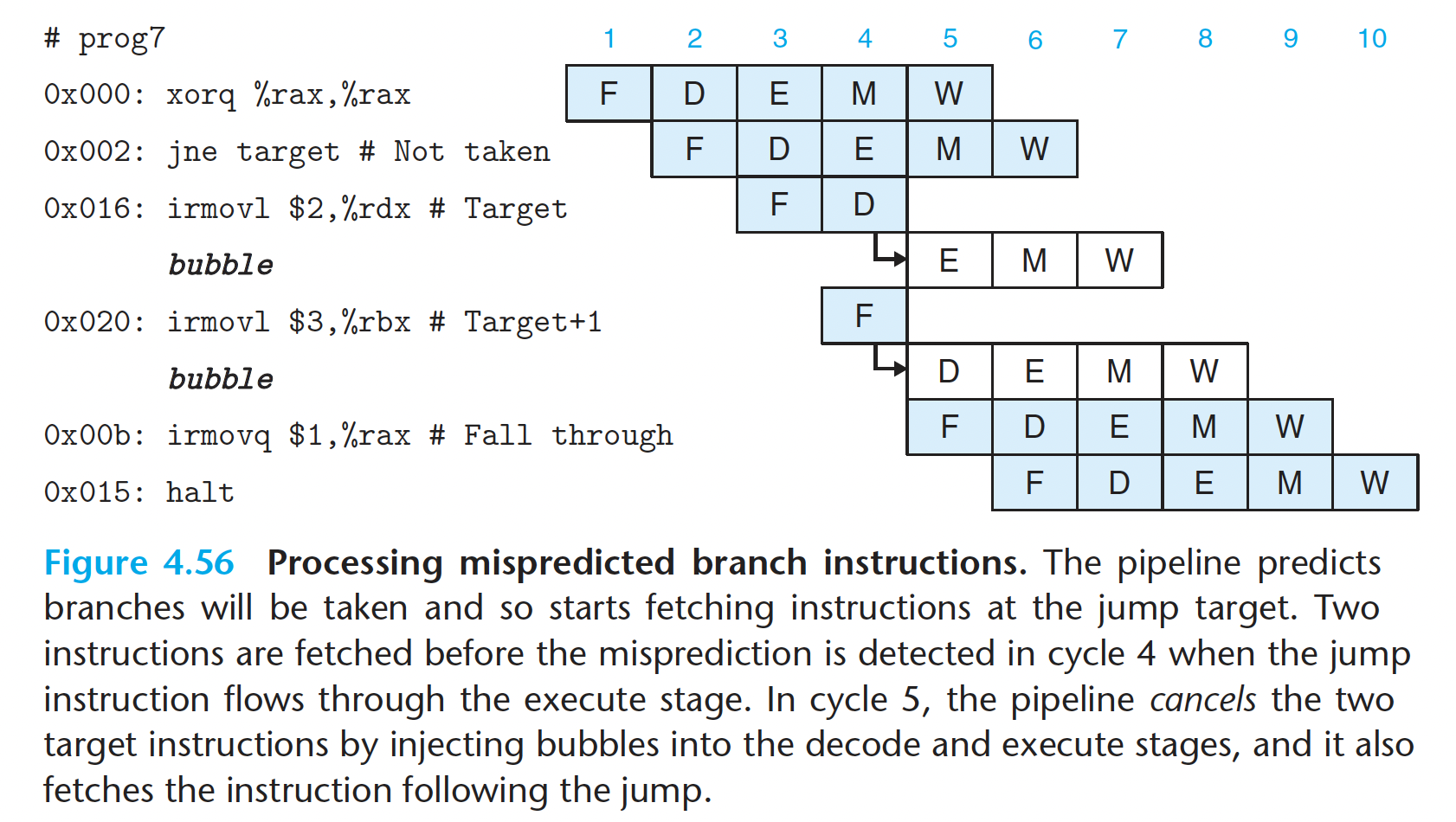
要处理预测错误的分支,考虑下面这个用汇编代码表示的程序:
1 | 0x000: xorq %rax,%rax |
4.5.6 异常处理
内部异常:
- halt 指令
- 有非法指令和功能码组合的指令
- 取指或数据读写试图访问一个非法地址
4.5.7 PIPE 各阶段的实现
比较一下 SEQ 中产生 srcA 信号的逻辑的 HCL 代码与 PIPE 中相应 的代码:
1 | Code from SEQ |
- PC选择和取指阶段
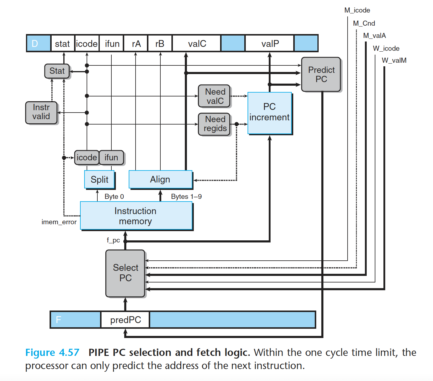
PC 选择逻辑从三个程序计数器源中进行选择。当一条预测错误的分支进入访存阶段时,会从流水线寄存器 M( 信号 M_valA) 中读出该指令 valP 的值(指明下一条指令的地 址)。当 ret 指令进入写回阶段时,会从流水线寄存器 W(信号 W_valM)中读出返回地址。 其他情况会使用存放在流水线寄存器 F(信号 F_predPC) 中的 PC 的预测值:
1 | word f_pc = [ |
当取出的指令为函数调用或跳转时, PC 预测逻辑会选择 valC, 否则就会选择 valP:
1 | word f_predPC = [ |
Practice Problem 4.30
Write HCL code for the signal f_stat, providing the provisional status for the fetched instruction.
1 | word f_stat = [ |
- 译码和写回阶段
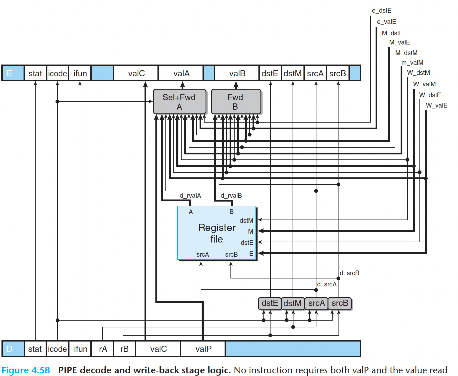
图 4-58 是 PIPE 的译码和写回逻辑 的 详 细说 明。标号为 “ctstE”、 “ctstM”、 “srcA” 和 “srcB” 的块非常类似于它们在SEQ的实现中的相应部件。 我们观察到,提供给写端 口的寄存器 ID 来 自于写回阶段(信号 W_dstE 和 W_dstM), 而不是来自于译码阶段 。 这是因为我们希望进行写的目的寄存器是由写回阶段中的指令指定的 。
流水线寄存器 E 的 valA 新值的 HCL 描述 :
1 | word d_valA = [ |
Practice Problem 4.34
Write HCL code for the signal d_valB, giving the value for source operand valB supplied to pipeline register E.
1 | word d_valB = [ |
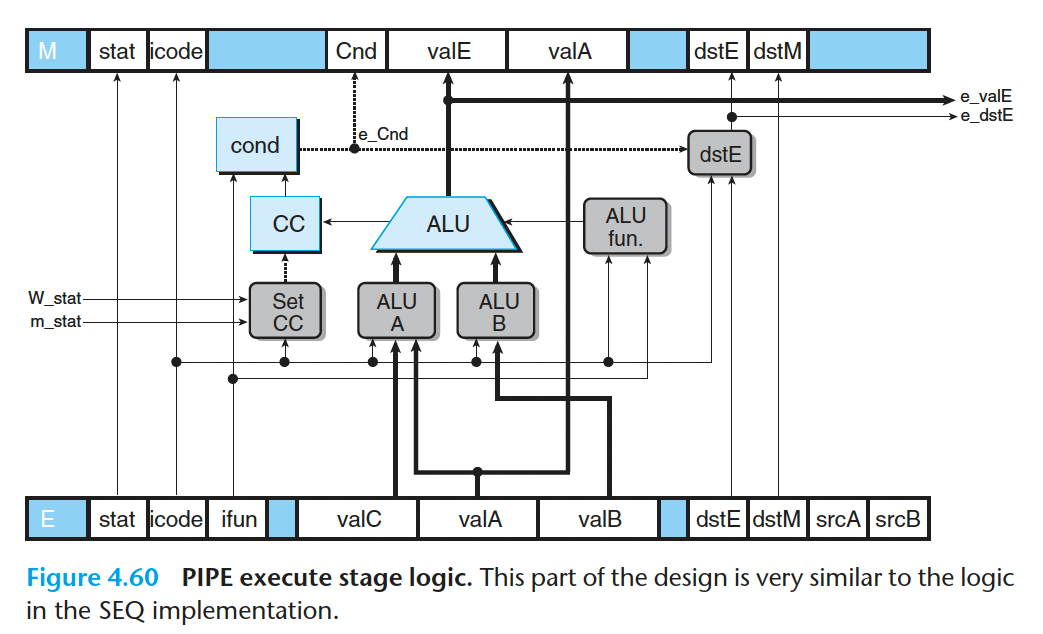
- 执行阶段
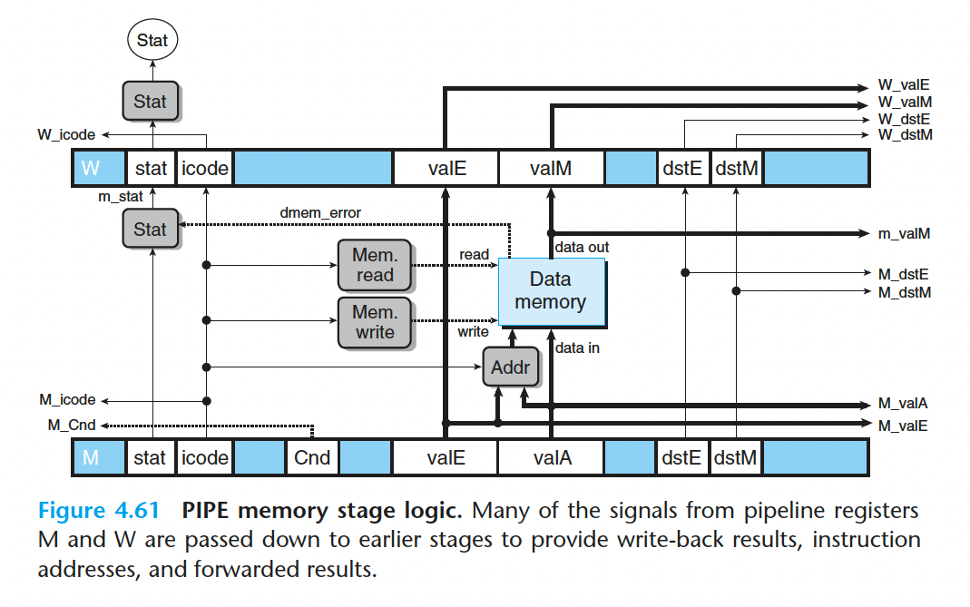
- 访存阶段
4.5.8 流水线控制逻辑
略